Errors in the data are inevitable and can be considered in terms of accuracy and precision.

Accuracy is a particular problem in occupancy analytics because almost all of the available data is coming from proxy sources (see the previous section on Measurement).

By definition, a proxy is measuring something indirectly: measuring the proxy provides data that can be used to infer the underlying measurement we are interested in.

However, this process of inference must be carefully considered, and take into account that semantically identical inputs from the perspective of our intended measurement may not result in identical outputs from the proxy.

For example, suppose we are attempting to measure the Physical Occupancy of a building, and to do so we have chosen the Access Control System (ACS) as our proxy. This proxy was chosen based on the following hypothesis:

Now imagine an employee – Jane – arriving at this zone and finding that her badge is not working. Perhaps Jane would see a receptionist who would check her id and then open the visitor gate for her. Such an event would not be automatically tracked as “Jane entering” by the proxy measurement and so Jane would continue to be considered outside/not physically occupying the building, despite the underlying semantic input being identical to her obtaining access with her own working badge: namely Jane has entered the building.

Another example might be that there is a rear exit to the building which does not require a badge to be presented. Anyone leaving via this exit will continue to be counted as Physically Occupying the building because the most recent ACE event associated with their badge will remain their entry to the building.

Proxies are almost inevitably subject to these kinds of inaccuracies, but they are rarely properly understood.

In most occupancy analytics, the largest contributions to inaccuracy are:

• The absence of a sufficiently clear Proxy Hypothesis; and
• Inadequate or incomplete assessment of the factors – both intrinsic (caused by the system itself or how it is configured) or extrinsic (caused by the way the system is then used) – affecting the accuracy of the proxy.

However, even highly accurate measurements may still lack precision:

Many proxies have limitations in their precision that are material to occupancy analysis. The most obvious examples are indoor positioning systems, where a subject in a specific, fixed location may be reported in a range of locations (though hopefully nearby!) without actually moving.

However, one of the complexities of occupancy analysis is that the proxies are either not designed well for error detection and correction, or not designed with this in mind at all.

This is often manifest by the proxy attempting some form of simplistic error correction without a clear Proxy Hypothesis or adequate identification of factors that will impair the accuracy, or understanding the nature of the imprecision.

For example, Presence Sensors (for example Passive InfraRed – PIR – sensors) fire events in real-time when they detect motion. However, these sensors are also intrinsically subject to misreporting (typically under-reporting) because their sensitivity is set to avoid false-positives (i.e. reporting presence when there is none). This means that inevitably some presence in not detected. To compensate for this, the sensors themselves often conduct local processing to report in some period – perhaps 1 minute. The sensor will report occupancy for that minute if at any point during the minute a presence event occurs, and will report no occupancy if there are no presence events.

There are two problems with these kind of systematic corrections:

• Without properly understanding the underlying threshold for a correct reading, it isn’t possible to determine whether the correction is leading to accurate, under- or over-reporting of the underlying measurement. Again in the PIR example, the trigger threshold may be such that many people can sit sufficiently still to go undetected for long periods of time, resulting in the system under-reporting actual presence, but on the other hand someone who spends most of their time moving around the office and only comes back to a space they are using for 5 seconds every couple of minutes could be being reported as continuously present, resulting in over-reporting of the actual presence.
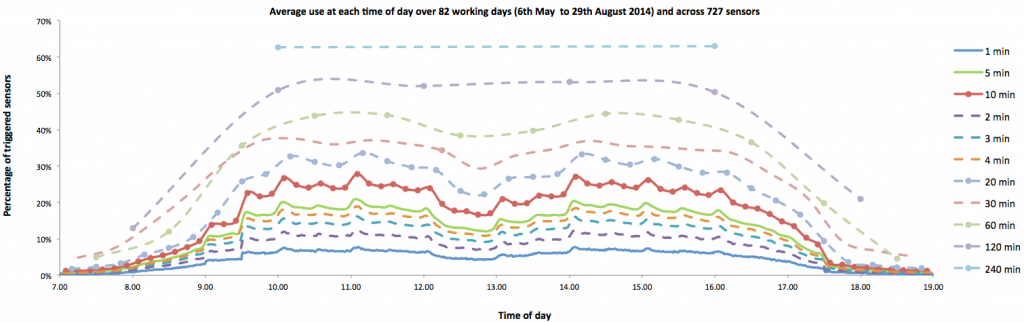
• The correction itself may introduce an arbitrary bias in reporting. Again, using the PIR example, the choice of 60 seconds for the reporting period is arbitrary. Most of these PIR sensor systems further aggregate presence data into longer reporting periods – often 10 minutes, 15 minutes or 1 hour. However, the choice of aggregation period dramatically affects the result of the measurement. or example, consider the extreme case of of someone who walks up to a desk to remove a coffee mug they noticed had been left on it. If that desk was not used for the remainder of the 9am – 5pm day, then the 1 minute aggregation (assuming the presence was indeed detected) would show 1/480th or 0.2% Utilization of Capacity for that desk. At a ten minute aggregate, that same event would be reported as 1/48 or 2% utilization. Hourly reporting would show 11%, and at a daily level that desk would be shown as fully occupied. The chart below shows the impact of this effect on real data from an office instrumented with 727 passive infrared sensors. Each curve represents a different aggregation interval of exactly the same sensor data, and as can be seen, the choice of the aggregation interval alone results in reported ‘occupancy’ ranging from less than 10% (at 1 minute/no aggregation) to over 60% (at 4 hour aggregation).

Having defined accuracy and precision and understood some of the common causes of these errors, there remains a key question: how can errors be detected in the data?

There are three fundamental types of error detection:

1. Comparison to known good data
2. Reasonableness testing
3. Correlation with other proxies

Comparison

Although an extremely convincing method of error detection, comparison is often difficult to perform. As previously described, occupancy measurements are very difficult to obtain directly, and any alternative indirect method of measurement (perhaps involving a different proxy) is susceptible to its own errors.

Comparison is therefore only viable in cases where the required measurement can be established using a practical, direct and error-free (or error-correctable) method that is sufficient to allow comparison with the corresponding proxy data. This is often not possible: indeed, if such a direct measurement method exists, then it would normally be used in place of the proxy.

Therefore, comparison is typically only used where it is feasible to undertake a short-duration or limited extent direct measurement that can be used for the purpose of testing the proxy. For example, it may be possible to have someone at each ACS entry point to manually count people arriving or leaving everyday for a week. Similarly, PIR sensors in an area of an office could be subjected to continuous observation and records kept of the times at which people arrive at or leave each individual space (for example each workstation). These direct measurements through observation are too expensive to continue permanently, but can be used to check the data being reported by the respective proxy (ACS or PIR).

Care must be taken when checking the proxy data in this way that the tests conducted are representative of the identified factors that may lead to inaccuracy or imprecision, and that verify the extent to which the Proxy Hypothesis is indeed true. For example, observing a block of workstations and concluding that the PIR sensors attached to them were providing accurate and precise data about the Utilization of Capacity could not be generalized to infer the reliability of PIR in a different setting (e.g. for measuring Utilization of Capacity of meeting rooms).

Reasonableness

There are many cases where data cannot realistically or practically be checked, and where the ‘correct’ data cannot therefore be established. However, this does not mean that errors can’t be identified.

The first method for identifying errors in these circumstances is reasonableness testing. As the name suggests, these test whether or not the data being received seems to be reasonable, and if not, the data can be flagged as suspect – perhaps leading to a more detailed examination.

Reasonableness tests depend on the specific measurement being tested. These tests tend to take one of two forms:

1. Ratio – where two independent measurements are compared to one another to see if the result is realistic. For example, dividing the Area taken up by workstation spaces by the number of workstations (Resource Count) gives the area per workstation. A reasonableness test of this ratio might be that it is 3sqm (30sqft). If data is measured – say from a CAFM system – that is less than 3sqm then that suggests that either the Area is being under-reported or the number of workstations is being over-reported.
2. Trend – this compares a measurement to the other recent measurements of the same item. For example, global Headcount might be measured monthly and a movement in one month of more than 1% might suggest that some misreporting has taken place. In this example, it is easy to see that reasonableness testing doesn’t necessary identify an error, it only shines a light on data that is suspect: the Headcount might have changed significantly from one month to the next if there had been a corporate acquisition or significant redundancies.

Correlation

The third technique for detecting errors is to exploit correlation between otherwise independent proxies. If two proxies provide the same inferred measurement and the proxies themselves are independent of one another, the the confidence in the accuracy and precision of that measurement are increased.

For example, a common scenario is to use the correlation between ACS activities, reservation check-ins and network connections (IPDD) to more accurately infer Physical Occupancy. In the example above where Jane’s security badge fails, she would almost certainly still connect her computer to the network once in the office, and check-in to any reservations she had made that day. By correlating the IPDD and reservation data her Physical Occupancy could be inferred with fairly high confidence even though the ACS proxy reported her as not present.

This is a very powerful method of error detection.

However, care must be taken to ensure that the proxies involved are truly independent. Suppose, for example, that the ACS was connected to the Reservation Management System so that when someone badged-in to the building they were automatically checked in to all of their reservations for that day. Now suppose that on another day, Jane had planned to work in the office and made reservations for a workstation and a booth for a conference call she had, but at the last minute needed to go and visit a client. Jane needed an information pack from the office so she went in early, picked up the pack, and headed out to see the client, not returning to the office. In this case, the ACS would report a badge-in, and – because of the automation – this ACS event would automatically also check-in Jane’s workstation and telephone booth reservations for that day. When processing this data, both the ACS and Reservation Management Systems would be reporting Jane as present, and only the IPDD system would be reporting her as not present, so using a simple majority rule the data would report Jane as physically occupying the building that day.

Three methods are generally viable for correcting errors in occupancy data:

1. Correlation inference
2. Reasonableness and manual intervention
3. Accuracy correction for precise data

Correlation inference

This method uses multiple proxies to attempt to make the same measurement, and then applying a specific rule or heuristic to determine the safest inference that can be made.

For example, a Reservation Management System and IPDD may both be used to measure Physical Occupancy of specific reservable workstations. If the Reservation Management System reports a reservation for a specific person, and that person’s laptop is also reported by IPDD as being docked during the same period as the reservation, then this complete correlation gives very high confidence in the inference that this person Physically Occupied this workstation during the period.

On the other hand, if the IPDD reported use of the reserved workstation until an hour after the reservation ended, and in the absence of any user initiated “extend reservation” event, then a rule may be applied that states that the continued IPDD presence events for this houe indicates continued Physical Occupancy, notwithstanding the reservation terminating.

Similarly, if both Reservation Management and IPDD reported presence at the same times, but at different workstations, it is likely that a rule would infer the actual Physical Occupancy Space from the IPDD data rather than the reservation data.

Note, however, that these examples are also only inferences with varying degrees of confidence – it isn’t possible to know from the data alone what the person was actually doing, as neither proxy tells us that.

Reasonableness and manual intervention

Once reasonableness test have been introduced, they are most commonly used to highlight suspect data and initiate a process of manual intervention to try to understand why the data failed the reasonableness test.

This might involve establishing the wider context of the anomaly. For example, a spike in building Physical Occupancy might be caused by an all-hands meeting, and therefore the data is correct, just unusual. See also the Unintended consequences story.

It is good practice, when a reasonableness test fails, and the cause is established, to review and if possible refine the reasonableness test to make it stronger. For example, if all-hands meetings were published on a system somewhere, this system could be automatically checked when occupancy peaks were detected to see if there was an all-hands meeting on that day, and the tolerances for what constitutes and “unreasonable” peak adjusted accordingly.

Accuracy correction for precise data

This third method of error correction is included to deal with proxies that have high precision (i.e. they always produce the same outputs for a given semantically equivalent input) but low accuracy.

To help picture such a system, imagine a crossbow with a scope and every time it is fired with the sight perfectly central on the bullseye, the arrow hits the target in the exact same spot 20 cm above the bullseye. This crossbow is inaccurate but very precise. Clearly, in this case, the scope would be adjusted so that it was both accurate and precise.

However, in the world of occupancy, the proxies that provide the data are often “adjusted” for some other primary purpose – secure access control, network access etc. – and so there is limited opportunity to re-calibrate them.

Instead, the outputs can be adjusted. In the crossbow example, this is a bit like moving the target after the arrow is fired. As long as the proxy is precise, a compensating adjustment can be used to adjust the output data to make it more accurate.

How accurate the results become depends on the reliability of the compensating adjustment. For example, a high precision ACS might only provide information about people entering the building who have been issued with a security badge of their own. If the Physical Occupancy of the building is required, then this cohort is only part of the total – there will also be visitors who either don’t have a badge at all (e.g. from another organization) or whose badge does not grant them access to this building (for example colleagues from another location). It may be possible to establish via a study that these additional non-badge holding occupants consistently number between 4% and 6% of the badge-holding occupants on any one day. With this information, the ACS data could simply be inflated by 5% and the new figure would now be bothe precise and accurate (assuming that the ACS was precise in the first place, which is a big assumption!)

The potential errors in any data source must be carefully considered. For each measurement that is sought, a Proxy Hypothesis should be established, and the factors affecting accuracy and precision should be documented.

Once the proxy is selected, a testing regime should be put in place to continuously monitor data from the proxy using comparison, reasonableness and/or correlation techniques.

Data that is determined to be questionable should be subjected to corrections using correlation inference, unreasonable data manual intervention and/or accuracy correction for precise data.

Having defined these steps, the level of confidence in each measurement that is being used for subsequent analysis must be reviewed. This may be expressed as a confidence interval (e.g. +/- 10%), as a statistical deviation (e.g. standard deviation of 100) or in some other way.

The level of confidence of the measurements that are used in an analysis can become compound, and so just because each individual measurement may have a relatively small confidence interval, a compound metric based on multiple measurements might have a far larger confidence interval.